Time ranges and the atmospheric response

Script showing how a user might want to consider choosing their analysis time range in relation to the atmospheric response.

Check out the Choosing a time range section in the online documentation for more details on other observational time range factors to consider.

Throughout FOXSI-4’s flight, there are different amounts of atmosphere in the line of sight that will attenuate the incoming X-rays. This example will show how to get to the atmopspheric response values.

The example originally followed the plot produced from response_tools.attenuation.asset_atm().

Note: The atmospheric response is included in the level 3 ARF response functions that have “flight” in their name. E.g, response_tools.responses.foxsi4_telescope0_flight_arf which will require a time_range input to work.

from astropy.time import Time
from astropy.visualization import time_support
import astropy.units as u
from matplotlib.dates import DateFormatter
import matplotlib.pyplot as plt
import numpy as np

from response_tools.attenuation import att_foxsi4_atmosphere

time_support()

<astropy.visualization.time.time_support.<locals>.MplTimeConverter object at 0x7ffbb945ffe0>

The function documentation

The documentation for any function in response-tools can be found online here.

The response_tools.attenuation.att_foxsi4_atmosphere documentation can be found here, but we can also use the help function.

help(att_foxsi4_atmosphere)

Help on function att_foxsi4_atmosphere in module response_tools.attenuation:

att_foxsi4_atmosphere(mid_energies, time_range=None, file=None)
    Atmsopheric attenuation from and for FOXSI-4 flight data.

    Parameters
    ----------
    mid_energies : `astropy.units.quantity.Quantity`
        The energies at which the transmission is required. If
        `numpy.nan<<astropy.units.keV` is passed then an entry for all
        native file energies are returned.
        Unit must be convertable to keV.

    time_range : `astropy.units.quantity.Quantity` or `None`
        The time range the atmsopheric transmissions should be averaged
        over. If `None`, `numpy.nan<<astropy.units.second`, or
        `[numpy.nan, numpy.nan]<<astropy.units.second` then the full
        time will be considered and the output will not be averaged but
        a grid of the transmissions at all times and at any provided
        energies. Should be of length 2. Can be given as seconds since
        launch or as UTC time as well either as a string or and Astropy
        time.
        - Observation start: 100<<astropy.units.second
        - Observation end: 461<<astropy.units.second
        - String format: YYYY-mm-ddTHH:MM:SS
        - Observation start: 2024-04-17T22:14:40
        - Observation end: 2024-04-17T22:20:41

    file : `str` or `None`
        Path/name of a custom file wanting to be loaded in as the
        atmospheric data file.

    Returns
    -------
    : `AttOutput`
        An object containing the energies for each transmission, the
        transmissions, and more. See accessible information using
        `.contents` on the output.

    Example
    -------
    >>> from astropy.time import Time
    >>> import astropy.units as u
    # two equivalent calls to the function
    # using Astorpy times
    >>> a0 = att_foxsi4_atmosphere([np.nan]<<u.keV,
                                   time_range=Time(["2024-04-17T22:14:40",
                                                    "2024-04-17T22:20:41"],
                                                   format='isot',
                                                   scale='utc'))
    # using seconds from launch values (unit-aware)
    >>> a1 = att_foxsi4_atmosphere([np.nan]<<u.keV,
                                   time_range=[100,
                                               461]<<u.second)

Using the function

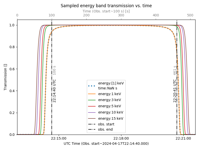
Here it is seen the function would like energies and a time range. A user can also see there are some helpful time markers like the observation start (shutter door open) and observation end (shutter door closed). Notice these times are slightly early and late of the first and last time interval shown in the Choosing a time range table, respectively.

Before getting into time ranges, a user might want to only sample one energy, or several, and inspect the time profile of the attenuation.

To get all times back from the function, specific times don’t need to known. The function will return all times if numpy.nan is passed (but it still needs to be unit-aware).

So let’s get the atmsopheric transmission at 1 keV for the full flight:

energy0, time0 = [1]<<u.keV, np.nan<<u.second
atm0 = att_foxsi4_atmosphere(mid_energies=energy0,
                             time_range=time0)

Now atm0 stores the transmission time rpofile for 1 keV photons.

A user might want to inspect the time profile for several energies. To do this, an energy array can be passed which will return a matrix in the transmission attribute where the rows are times and the columns are the different energy transmissions.

energy1 = [1, 3, 5, 10, 15]<<u.keV
atm1 = att_foxsi4_atmosphere(mid_energies=energy1,
                             time_range=time0)

A user will likely want to select times out of the time profile, so let’s start defining some times in which a user might be interested. Say, the time range spanning the whole observation time:

# in seconds since launch
obs_start2end_sec = [100, 461] << u.second
# in UTC
obs_start2end_utc = Time(["2024-04-17T22:14:40",
                          "2024-04-17T22:20:41"],
                         format='isot',
                         scale='utc')

Atmospheric transmission time profile

This information can be visualised (although plotting code always looks messy):

fig = plt.figure(figsize=(8,6))
gs_ax0 = plt.gca()

# transmissions from only passing one energy
p0 = gs_ax0.plot(atm0.times_utc,
                 atm0.transmissions,
                 ls=":",
                 label=f"energy:{energy0:latex}\ntime:{time0:latex}",
                 lw=3)
# plot the different energy transmission time profiles
p1 = []
for i in range(len(energy1)):
    p1 += gs_ax0.plot(atm1.times_utc,
                      atm1.transmissions[:,i],
                      ls="-",
                      label=f"energy:{energy1[i]:latex}")

# label bookkeeping
gs_ax0.set_ylabel(f"Transmission [{atm0.transmissions.unit:latex}]")
gs_ax0.set_xlabel(f"UTC Time (Obs. start~{obs_start2end_utc[0]})")
gs_ax0.set_ylim([0,1.05])
gs_ax0.set_xlim([atm1.times_utc[0], atm1.times_utc[-1]])
gs_ax0.set_title("Sampled energy band transmission vs. time")
gs_ax0.xaxis.set_major_formatter(DateFormatter("%H:%M:%S"))
# would like to display seconds since launch along the top of the plot
gs_ax0b = gs_ax0.twiny()
gs_ax0b_color = "grey"
_ = gs_ax0b.plot(atm0.times, atm0.transmissions, lw=0)
v0 = gs_ax0b.axvline(obs_start2end_sec[0].value, ls="-.", c="k", label="obs. start")
v2 = gs_ax0b.axvline(obs_start2end_sec[-1].value, ls="-.", c="k", label="obs. end")
gs_ax0b.set_xlabel(f"Time (Obs. start~100 s) [{atm0.times.unit:latex}]", color=gs_ax0b_color)
gs_ax0b.set_xlim([atm1.times[0].value, atm1.times[-1].value])
gs_ax0b.tick_params(axis="x", labelcolor=gs_ax0b_color, color=gs_ax0b_color, which="both")
# let's put the timestamps on the plot
_y_time_loc = 0.3
_x_offset = 4 << u.second
gs_ax0.annotate(f"{obs_start2end_utc[0].strftime('%H:%M:%S')} UTC", (obs_start2end_utc[0]+_x_offset, _y_time_loc), rotation=90)
gs_ax0.annotate(f"{obs_start2end_utc[-1].strftime('%H:%M:%S')} UTC", (obs_start2end_utc[-1], _y_time_loc), rotation=90, ha="right")
_y_sec_loc = _y_time_loc+0.25
gs_ax0b.annotate(f"{obs_start2end_sec[0]:.0f}", (obs_start2end_sec[0].value+_x_offset.value, _y_sec_loc), color=gs_ax0b_color, rotation=90)
gs_ax0b.annotate(f"{obs_start2end_sec[-1]:.0f}", (obs_start2end_sec[-1].value, _y_sec_loc), color=gs_ax0b_color, rotation=90, ha="right")
# make sure to show the legend
plt.legend(handles=p0+p1+[v0,v2])
plt.tight_layout()
plt.show()

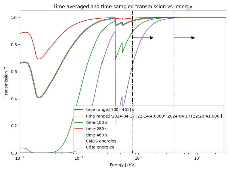
Atmospheric transmission for a time range

A user can decide they do not care about the energy range for the transmission. (Note: this should be decided by the RMF.)

Similar to what was seen for the time_range input, numpy.nan can be passed (unit-aware). Let’s average over the whole time range:

energy2 = np.nan<<u.keV
atm2 = att_foxsi4_atmosphere(mid_energies=energy2,
                             time_range=obs_start2end_sec)

Since the time_range can be given as seconds since launch and in Astropy UTC, the following code is equivalent to the above for atm2:

atm2a = att_foxsi4_atmosphere(mid_energies=energy2,
                              time_range=obs_start2end_utc)

A user can also just return all transmissions at all energies and times from the original file containing the data:

energy3, time3 = np.nan<<u.keV, np.nan<<u.second
atm3 = att_foxsi4_atmosphere(mid_energies=energy3,
                             time_range=time3)

This can be plotted of course to get a better idea of what is going on.

Let’s plot the averaged transmissions over the whole observation at the native file energy resolution (atm2) and then let’s use atm3 to sample some transmission curves at some “random” instantaneous times by indexing.

Let’s mark where the CdTe and CMOS detector telescope energies ranges lie on the plot for more context.

fig = plt.figure(figsize=(8,6))
gs_ax1 = plt.gca()

# whole time range average
p2 = gs_ax1.plot(atm2.mid_energies,
                 atm2.transmissions,
                 ls="-",
                 lw=3,
                 label=f"time range:{obs_start2end_sec:latex}")
p2a = gs_ax1.plot(atm2a.mid_energies,
                  atm2a.transmissions,
                  ls="-.",
                  label=f"time range:{obs_start2end_utc}")
# random instantaneous times
p3 = gs_ax1.plot(atm3.mid_energies,
                 atm3.transmissions[:, 2000],
                 ls="-",
                 label=f"time:{atm3.times[2000]:latex}")
p4 = gs_ax1.plot(atm3.mid_energies,
                 atm3.transmissions[:, 5600],
                 ls="-",
                 label=f"time:{atm3.times[5600]:latex}")
p5 = gs_ax1.plot(atm3.mid_energies,
                 atm3.transmissions[:, 9200],
                 ls="-",
                 label=f"time:{atm3.times[9200]:latex}")

# let's show the CdTe and CMOS energies on this plot for conntext
cmos_le = 0.8<<u.keV
v3 = gs_ax1.axvline(cmos_le.value, ls="-.", c="k", label="CMOS energies")
gs_ax1.arrow(cmos_le.value, 0.85, 1, 0, length_includes_head=True, head_width=0.02, head_length=0.2, color="k")
cdte_le = 4<<u.keV
v4 = gs_ax1.axvline(cdte_le.value, ls=":", c="k", label="CdTe energies")
gs_ax1.arrow(cdte_le.value, 0.85, 5, 0, length_includes_head=True, head_width=0.02, head_length=1, color="k")
# some label bookkeeping
gs_ax1.set_ylabel(f"Transmission [{atm3.transmissions.unit:latex}]")
gs_ax1.set_xlabel(f"Energy [{atm3.mid_energies.unit:latex}]")
gs_ax1.set_ylim([0,1.05])
gs_ax1.set_xlim([0.01, 30])
gs_ax1.set_xscale("log")
gs_ax1.set_title("Time averaged and time sampled transmission vs. energy")
plt.legend(handles=p2+p2a+p3+p4+p5+[v3,v4])
plt.tight_layout()
plt.show()

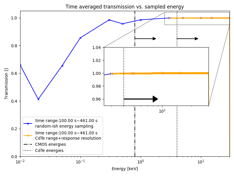
Atmospheric transmission with different energy resolutions

From the above plot, the user can see quite a bit of detail in the time profiles but a user will likely wish to match the energy resolution to that of the relevant telescope RMF.

So, let’s show the full observation time curve with different energy resolutions:

# some random energies
energy4 = [0.01, 0.02, 0.05, 0.1, 0.3, 0.5, 1, 3, 5, 10, 15, 30]<<u.keV
atm4 = att_foxsi4_atmosphere(mid_energies=energy4,
                             time_range=obs_start2end_sec)

Let’s also consider the CdTe RMF energy resolution:

energy5 = np.arange(3,30.1, 0.1)<<u.keV
atm5 = att_foxsi4_atmosphere(mid_energies=energy5,
                             time_range=obs_start2end_sec)

Let’s plot this to see how it looks:

fig = plt.figure(figsize=(8,6))
gs_ax2 = plt.gca()

# random energy resolution
colour4 = "blue"
p6 = gs_ax2.plot(atm4.mid_energies,
                 atm4.transmissions,
                 label=f"time range:{atm4.times[0]:.2f}$-${atm4.times[-1]:.2f}\nrandom-ish energy sampling",
                 marker="x",
                 ms=4,
                 c=colour4)
# CdTe energy resolution
colour5 = "orange"
gs_ax2.plot(atm5.mid_energies,
            atm5.transmissions,
            label=f"time range:{atm5.times[0]:.2f}$-${atm5.times[-1]:.2f}\nCdTe range+response resolution",
            marker="x",
            ms=2,
            c=colour5)

# add the lowest energies of the detectors
v5 = gs_ax2.axvline(cmos_le.value, ls="-.", c="k", label="CMOS energies")
gs_ax2.arrow(cmos_le.value, 0.85, 1, 0, length_includes_head=True, head_width=0.02, head_length=0.2, color="k")
v6 = gs_ax2.axvline(cdte_le.value, ls=":", c="k", label="CdTe energies")
gs_ax2.arrow(cdte_le.value, 0.85, 5, 0, length_includes_head=True, head_width=0.02, head_length=1, color="k")

# inset Axes for the CdTe plot
x1, x2, y1, y2 = 2.5, 30, 0.95, 1.04  # subregion of the original image
axins = gs_ax2.inset_axes([0.4, 0.35, 0.5, 0.4],
                            xlim=(x1, x2),
                            ylim=(y1, y2)) #, xticklabels=[], yticklabels=[])
axins.plot(atm4.mid_energies, atm4.transmissions, label=f"time range:{atm4.times[0]:.2f}$-${atm4.times[-1]:.2f}\nrandom-ish energy sampling", marker="x", ms=6, c=colour4)
p7 = axins.plot(atm5.mid_energies, atm5.transmissions, label=f"time range:{atm5.times[0]:.2f}$-${atm5.times[-1]:.2f}\nCdTe range+response resolution", marker="x", ms=4, c=colour5)
axins.set_xscale("log")
_rectangle, _connectors = gs_ax2.indicate_inset_zoom(axins, edgecolor="black")
# edit the connecting lines so they make sense
_connectors[0].__dict__["_visible"] = False
_connectors[1].__dict__["_visible"] = True
# add the lowest energies of the detectors to the inset plot
_ = axins.axvline(cmos_le.value, ls="-.", c="k", label="CMOS energies")
axins.arrow(cmos_le.value, 0.96, 1, 0, length_includes_head=True, head_width=0.01, head_length=0.2, color="k")
_ = axins.axvline(cdte_le.value, ls=":", c="k", label="CdTe energies")
axins.arrow(cdte_le.value, 0.96, 5, 0, length_includes_head=True, head_width=0.01, head_length=1, color="k")

# some label bookkeeping
gs_ax2.set_ylabel(f"Transmission [{atm3.transmissions.unit:latex}]")
gs_ax2.set_xlabel(f"Energy [{atm3.mid_energies.unit:latex}]")
gs_ax2.set_ylim([0,1.05])
gs_ax2.set_xlim([0.01, 30])
gs_ax2.set_xscale("log")
gs_ax2.set_title("Time averaged transmission vs. sampled energy")
plt.legend(handles=p6+p7+[v5,v6])
plt.tight_layout()
plt.show()

/home/runner/work/response-tools/response-tools/examples/plot_atmospheric_response.py:300: MatplotlibDeprecationWarning: Since Matplotlib 3.10 indicate_inset_[zoom] returns a single InsetIndicator artist with a rectangle property and a connectors property.  From 3.12 it will no longer be possible to unpack the return value into two elements.
  _rectangle, _connectors = gs_ax2.indicate_inset_zoom(axins, edgecolor="black")

It can be seen that the resolution smooths over a lot of the behavious and it can also be seen that the atmosphere has very little effect in the CdTe energy range.