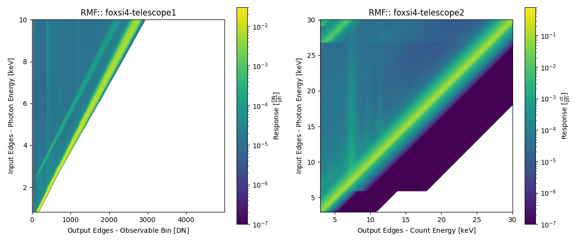
Example FOXSI-4 RMFs

Script showing a quick example how to obtain and plot the Redistribution Matrix Functions (RMFs) for a Hard and Soft X-ray (H/SXR) FOXSI-4 telescope.

The chosen SXR and HXR telescopes are Telescope 0 and 2, respectively. Telescope 0 utilizes a CMOS detector and Telescope 2 has a CdTe Double-sided Strip Detector (CdTe-DSD).

For telescope components to choose, see the FOXSI-4 Instrumentation documentation

import astropy.units as u
from matplotlib.colors import LogNorm
import matplotlib.gridspec as gridspec
import matplotlib.pyplot as plt
import numpy as np

import response_tools.responses as responses

A note on usage and user options

One great thing about the unit-awareness of the inputs/outputs is that you can pass any reasonable input units and they’ll be converted for you so you don’t need to worry about conversion factors throughout your code to use the functions.

As other examples will likely go into more detail than here, to generate a telescope response you only need to make a few core decisions related to the FOXSI-4 observation and the data in which the user is interested.

Please look over the FOXSI-4 observation resources to add more context as to how a user might decide on their choice of the following parameters. Additionally, look over the FOXSI-4 instrumentation resources when deciding which functions to use.

These crucial choices will be:

• A source location to obtain:

  • A detector region.

• A time range during the flight.

• An energy array (sometimes).

For more detail on choices:

• A detector region (for CdTe, input: region xor pitch):

  • For CdTe Redistribution Matrix Function (RMF) code.

    • Of course, this should be consistent with the off axis angle being used.

  • Use either, not both, inputs:

    • An integer for region input in [0,1,2].

    • Astropy.units unit convertable to micrometers for pitch input in [60 um,80 um,100 um].

Choosing the RMF parameters

When it comes to the CdTe detectors a user needs to decide which detector region(s) their data comes from in order to obtain the correct RMF. The strips vary in pitch across the detector and have 3 different regions:

• Region 0, pitch 60 $mu$m

• Region 1, pitch 80 $mu$m

• Region 2, pitch 100 $mu$m

(For observational choices, see the FOXSI-4 Observation documentation)

Luckily, for CMOS, it is less complicated as the RMF does not vary across the detector so no choice on region is necessary.

Let’s assume the CdTe region the user wants is for data in the center of the detector and so pick region 0 (60 $mu$m):

user_region = 0 # equivalent to defining ``user_pitch=60<<u.um``

Getting the RMFs

Now that the user has made their choices, the RMFs for any telescope are easily obtained:

# CMOS RMF
pos0_rmf = responses.foxsi4_telescope0_rmf()
# CdTe RMF
# if pitch is defined instead, pass as ``responses.foxsi4_telescope2_rmf(pitch=user_pitch)``
pos2_rmf = responses.foxsi4_telescope2_rmf(region=user_region)

Exploring the RMF information

The Response-tools code tips section describes the fields a user might find in the returned data class; however, it is worth noting the very important energy information that comes with the RMF object.

The two fields, input_energy_edges and output_energy_edges, define the energies at which all other analysis components should be evaluated and compared.

For example, if an ARF (example) is also being created then this should be evaluated with respect to the input_energy_edges`, most like the bin mid-points. This is the same for model evaluation in, say, spectral fitting analysis. The output_energy_edges define the bins at which the data is taken and for which the data calibrated.

Plotting RMF products

This might be unlikely but a user can then, of course, plot the RMFs they have loaded in:

fig = plt.figure(figsize=(12, 5))
gs = gridspec.GridSpec(1, 2)

# CMOS, telescope 0 RMF
gs_ax0 = fig.add_subplot(gs[0, 0])
extent = [np.min(pos0_rmf.output_energy_edges.value),
          np.max(pos0_rmf.output_energy_edges.value),
          np.min(pos0_rmf.input_energy_edges.value),
          np.max(pos0_rmf.input_energy_edges.value)]
r = gs_ax0.imshow(pos0_rmf.response.value,
                origin="lower",
                norm=LogNorm(vmin=1e-7, vmax=3e-2),
                extent=extent,
                aspect=(extent[1]-extent[0])/(extent[3]-extent[2])
                )
cbar = plt.colorbar(r)
cbar.ax.set_ylabel(f"Response [{pos0_rmf.response.unit:latex}]")
gs_ax0.set_xlabel(f"Output Edges - Observable Bin [{pos0_rmf.output_energy_edges.unit:latex}]")
gs_ax0.set_ylabel(f"Input Edges - Photon Energy [{pos0_rmf.input_energy_edges.unit:latex}]")
gs_ax0.set_title(f"{pos0_rmf.response_type}:: {pos0_rmf.telescope}")

# CdTe, telescope 2 RMF
gs_ax1 = fig.add_subplot(gs[0, 1])
r = gs_ax1.imshow(pos2_rmf.response.value,
                origin="lower",
                norm=LogNorm(vmin=1e-7, vmax=8e-1),
                extent=[np.min(pos2_rmf.output_energy_edges.value),
                        np.max(pos2_rmf.output_energy_edges.value),
                        np.min(pos2_rmf.input_energy_edges.value),
                        np.max(pos2_rmf.input_energy_edges.value)]
                )
cbar = plt.colorbar(r)
cbar.ax.set_ylabel(f"Response [{pos2_rmf.response.unit:latex}]")
gs_ax1.set_xlabel(f"Output Edges - Count Energy [{pos2_rmf.output_energy_edges.unit:latex}]")
gs_ax1.set_ylabel(f"Input Edges - Photon Energy [{pos2_rmf.input_energy_edges.unit:latex}]")
gs_ax1.set_title(f"{pos2_rmf.response_type}:: {pos2_rmf.telescope}")

plt.tight_layout()
plt.show()

Lower level RMF access (Extra)

In the above example, the imaginary user has used the Level 3 API but the RMF/detector response can be accessed at the lower levels as well.

Level 2:

• response_tools.telescope_parts.foxsi4_position#_detector_response where # refers to the telescope position number of interest.

Level 1:

• CdTe: response_tools.detector_response.cdte_det_resp

• CMOS: response_tools.detector_response.cmos_det_resp

Level 0:

• f"{response_tools.responseFilePath}/detector-response-data/"